Brief Intro to Haskell
If you wanna checkout the workshop, it’s Here
Note: Some codes in this article may not be legal haskell codes, they are only used to explain some facts.
This article is not originally written by me, I just read some Haskell articles online and put them together:
Learn You a Haskell for Great Good!
Haskell is a declarative (functional) programming language. You know what is functional programming, how to use functions as first class values, writing recursive programs, doing function composition and currying/uncurrying, so I’ll skip that part. This introduction will start with some basic stuff like data type.
It’s all about Functions!
Get started with recursive pattern matching functions
When we talk about Haskell, the first that comes into out mind is definitely Functions!. Before we get into details of Haskell functions, let’s take a look like what functions are look like. Say we want to write a function that calculate xth number of a fibonacci series, it looks like following
-- This is a comment in Haskell

-- This is a function definition in Haskell
-- Num is type class which represents numbers
-- a is a class variable
-- fib takes an integer and returns a number
fib :: Num a => Integer -> a

-- We define two base cases for a fibonacci series
fib 1 = 1
fib 2 = 1

-- Do recursion
fib x = fib (x - 1) + fib (x - 2)
When we execute the function fib, Haskell simply match the argument from top to button and return the result we want, which is called pattern matching.
Improve functions by introducing extra arguments
The fib function that we defined above is quite bad because of
- Repeated computation
- Diversed stack growth
Therefore we are going to improve it like this
-- This function name is legal in Haskell
fib' :: Num a => a -> a -> Integer -> a

-- This time, we did tail recursion and prevent waste of computations
fib' x y 3 = x + y
fib' x y a =
    fib' y (x + y) (a - 1)

-- Then we wrap fib' function
fib 1 = 1
fib 2 = 1
fib x = fib' 1 1 x
Curried function
Officially, function in haskell takes only one argument and produce one output. But how is it possible that we define a function that accept arbitrary number of arguments, like fib' we used above? The answer to that question is currying. Think about following function
bigger :: (Ord a) => a -> a -> a
bigger a b
    | a > b = a
    | b > a = b
It simply pick a larger number between two and return it. It takes two arguments and return one. But if we look at it in this way ((bigger 1) 2)
it starts to become clearer: bigger is a function that takes an Ord argument and returns another function that takes one Ord and return an Ord, so that perfectly make sense that every function in Haskell takes one argument. The behavior that applying arguments to a function in this ‘Chained’ manner is what we called currying. It gives you the illusion that a function can actually take multiple arguments at the same time.
So there is a question, are bigger 1 and bigger 2 the same function? Well, it is hard to tell because we only talk about equality in type class Eq, but the answer to this question is obviously NO, because they behaves totally differently.
High order functions
We mentioned something like ‘returning a function’ or accepting a function as parameter. Yes, that’s what high order functions do. A function can take a function as argument and apply it to something. This is so easy that we won’t discuss in detail here. I believe that when you learn Java or Python, yu have already used this feature for many times.
Data type and type classes
data types are like structures that has multiple properties to it
type, data and newtype
At the beginning of this article, let’s make sure we don’t mess up some of the terminologies in Haskell in terms of data types. When we manipulate data types, there are three keywords that we might use, type, data and newtype.
The type keyword is nothing more than defining type synonyms for existing types, that is, you take a type, add a new name referring to it, then you can use the new name and original name interchangably.
type IntList = [Int]
let a = [1,2,3] :: IntList
let b = [1,2,3] :: [Int]
a == b

> True
The data keyword is used to create you own data types, which is quite straightforward:
type ID = Int
type Name = String
type DEAD = ()
data Person = Person ID Name
            | Dead
The newtype keyword is to wrap an existing type in a new defined type. The difference between type and newtype is that the type produces a synonym fro existing type, which means the new type is identical to original one, while newtype produces a new type. In fact, newtype is like a special kind of data which has only one constructor with only one field, but not exactly (There are differences in efficiency and lazyness).
newtype efficiency and lazyness
newtype is more efficient than data in terms of wrapping types. With data keyword, you create a new data type, which brings overhead for wrapping and unwrapping operations. While with newtype, the Haskell knows the underlying type that you have wrapped, therefore the wrapped data can directly be referred to without extra overhead.
The newtype also has extra lazyness in it. Because Haskell has known the wrapped type and there is only one constructor with one fixed field, sometimes the construction is not necessarily evaluated in some cases (like pattern matching with wildcards). While using data, construction is evaluated everytime because there might be different constructors with unfixed fields, Haskell need to figure out which one to go with.
Now that we have understood some confusing terminologies, let’s dive into one of most things in Haskell, which is Functor.
Functors
Functor class in Haskell simply means something that can be mapped over with a function. Any instance of Functor must implement the fmap function
fmap :: Functor f => (a -> b) -> f a -> f b
where f is a wrapper for some value of any type, (a -> b) is simple a function that takes value of type a as a parameter and return value of type b. The fmap function applies the function to the value which is wrapped by f and produces a new value wrapped in the exact same form.
Differnt instances of functor have their implementations for fmap, for example, fmap of List is simply map, therefore the following statements are identical
fmap (1+) [1,2,3]
map (1+) [1,2,3]
Why functor?
When we use a programming language to interact with pieces of data to produce something that is useful, it’s hard to make sure everything is in the same data structure. Data is organized in different ways in differnt scenarios in order to achieve higher runtime or development efficiency. In order to manipulate all these different types of data, we want the programming language to gerneralize well, that is, we can perform similar actions to different types with a unified interface (Like Abstract Class and Interface in Java).
Think about the following scenario, we have a datatype constructed from a Tuple
data Student = Student {
    id :: Int,
    mark :: Int
}

buildFromTuple :: (Int, Int) -> Student
buildFromTuple (id, mark) = Student id mark
Then we want to create a list of Student type values from a list of tuples, we have
map buildFromTuple [(1,20),(2,57)]
which is intuitive. But what if the tuples are stored in other data structures like Vector? With the help of functor, we can simply unify the interface with fmap.
Type constructor being an instance of Functor
Type constructors can be functors. For instance, the Maybe type can be defined as
instance Functor Maybe where
    fmap _ Nothing = Nothing
    fmap f $ Just a = Just $ f a
Note that in the type definition of fmap, the wrapper f only takes one parameter as type parameter, therefore, the type constructor in implementations should take exact one parameter as well. Consider the Either type
instance Functor Either where
    fmap:: (a -> b) -> Either a -> Either b
This is incorrect, because the type constructor Either takes two parameters. In order to make it valid, simple partially apply the first parameter with a
instance Functor Either a where
    fmap :: (b -> c) -> Either a b -> Either a c
Function as an instance of Functor
Function is first class citizen in Haskell so it makes sense for it to be an instance of some Class. The function as a functor has the form (->) r. This can be simply treat as application of a function that takes exact one parameter (or wrap the parameter with this function). According the previous definition, the function Functor can be defined as
instance Functor ((->) r) where
    fmap f g = (\x -> f (g x))
In another word, fmap f g returns a function which takes a value x, apply g to it and apply f to the result. In order to explain why does this happen, we need to go back to the original definition of fmap function
fmap :: Functor f => (a -> b) -> f a -> f b
Replace f with (->) r in this case, we have
fmap :: (a -> b) -> ((->) r a) -> ((->) r b)
which is
fmap :: (a -> b) -> (r -> a) -> (r -> b)
It is obvious that the fmap function takes an function that takes a as parameter and return b, and a function takes r returns a and outputs a function takes r and returns b. So the second function is applied to r to get the result a then a -> b can be applied to a to get b.
Intuitively, this is function composition that we really love about in Haskell. So for function
fmap = (.)

-- The following equations are all equivalent
fmap a b
a . b
(.) a b
\x -> a $ b x
Functor Laws
In the above sessions, we discussed about the “Instance of Functor” instead of functor directly. The reason is that in order for an instance of Functor to be a functor, it need to obey functor rules which ensures calling a functor only maps a function over it without doing anything more. Here are the two rules
- If we map id function over a functor, the functor we get back should be the exact same one.
- Composing two functions and then map it over a functor is same as mapping one over it and then mapping another
Maybe is a functor, let’s see how it obeys the functor laws.
-- Law 1
fmap id Nothing = Nothing -- trivial
fmap id (Just x) = Just (id x) = Just x

-- Law 2
fmap (f . g) Nothing = Nothing
fmap (f . g) (Just x)
    = Just (f $ g x)
    = fmap f Just (g x)
    = fmap f (fmap g (Just x))
    = (fmap f) (fmap g (Just x))
There also examples that a type construct is an instance of a functor but isn’t an actual functor. Consider a data type with a counter which increases by one everytime fmap is applied to it.
data CtrMaybe a = CtrNothing
                | CtrJust Int a
                deriving (Show)

instance Functor CtrMaybe where
    fmap _ CtrNothing = CtrNothing
    fmap f $ CtrJust ctr x = CtrJust $ ctr + 1 $ f x
In this case, everytime the id function is mapped over the structure, the counter has increased by 1, which is not identical to previous one anymore (side effect). Therefore, this is not a functor.
Applicative Functors
In the cases we discussed above, we map a function that takes one paramter and produces one result over an instance of Functor to yield the exact same wrapper but with the value changed.
What if we have a function that accepts more than one parameter, for example (+) which takes two Num type values and add them together.
fmap (+) (Just 3) = Just ( (+) 3 )
We have a partially applied function wrapped in Just~ Let’s think about how we gonna use it. What everyone can simple see is that it is a functor, so one intuitive way of using it is to map a function over it. What can we do to a function with another function, well, simply apply the function in another function that takes a function as parameter.
fmap (\f -> f 3) a
-- For value wrapped in a, apply it to value 3
This sounds like trivial, but it does have some fancy usages in Haskell with the Applicative class.
Suppose that we have two numbers wrapped by a functor, Just 3 and Just 5, how do we add them together? As we previously discussed, we can use fmap with (+) to produce a functor wrapped function, then map over it with another value.
a = fmap (+) (Just 3)
fmap (\f -> f 5) a
Well, that looks really bad. You are using two lines of codes and an anonymous function in order for a task as simple as adding two numbers! That’s where Applicative Functor comes in.
In Applicative Functor, two new terms are introduced, which are pure and <*>. These two terms are not defined by default, the developer who defines the data type should implement them. The Applicative class can be defined as
class (Functor f) => Applicative f where
    pure :: a -> f a
    (<*>) :: f (a -> b) -> f a -> f b
It’s quite obvious from the class definition is that in order to be an instanve of Applicative, a variable need to be Functor first. The pure function takes a value of any type as parameter and return an applicative functor with the value in it. (Put the value in some sort of default context – a minimal context that still yields the value). The (<*>) extracts the function from the first functor and map over the second one.
For instance, the Maybe is a kind of Applicative Functor, which is defined as
instance Applicative Maybe where
    pure = Just
    Nothing <*> _ = Nothing
    Just f <*> something = f <$> something
With normal functor, you can only map a function over a functor without being able to get the result out of it or manipulate it. While Applicative Functor allows you to operate on several functors with a single function. Look at the following example:
pure (+) <*> Just 3 <*> Just 5
Just (3 +) <*> Just 5
The first line can be aggregated to the second one by paritally apply the plus to Just 3. Thanks to the unwrapping capability of <*> function, the wrapped function is easily unwrapped and applied. The good thing is that the second line has almost identical structure with the first one: Partially applying a wrapped function still yields a wrapped function, that why we can easily cascade multiple <*> functions.
If we generalize the usage of Applicative Functor, that becomes the following form
pure f <*> x <*> y <*> ...
Again, the strength of Applicative Functor over normal Functor is that it support function with any number of inputs and is able to cascade values in a fairly elegant manner.
The <*> has the pre-condition that the function is wrapped, which is not always necessary, say, if we just want to apply a function to a couple of wrapped values, there is no need to wrap the function up explicitly, that’s why the Applicative module introduces another function called <$>, which is exact same as fmap but has more elegant form when applied.
(<$>) :: Functor f => (a -> b) -> f a -> f b
For instance, if we want to apply (+) to Just 3 and Just 5, now we can simply write
(+) <$> Just 3 <*> Just 5
which is quite intuitive.
I think that’s some basic knowledge a beginner should know about Haskell before he actually start doing codes. In the following sections, I’ll talk about Haskell IO, datatypes, monads, something like that.
I/O
Haskell strictly separate pure codes and non-pure ones, which may cause the world to change. Therefore, a complete isolation of side-effects is provided from the language level, which is a nice feature that helps improve program stability, because many bugs in programs are caused by unanticipated side-effects.
Haskell I/O is a subset of those actions that might have side effect. Here are some examples of I/O functions
IO actions
putStrLn :: String -> IO ()
-- This writes out a string to standard output which an end-of-line char

getLine :: IO String
-- This gets a string from the standard input
Anything with IO Something in it is an IO action, which can be stored in a variable and evaluated later (because they are functions). They can also be glued toghther to form a larger block of action using do, like this
myblock = do
    putStrLn "Please type something"
    myStr <- getLine
Any IO action has an underlying data type bound to it, for example, the getLine function has a IO String in the type definition, which means it has a String value bound to it. Using <- when calling IO actions can get the underlying value and store it in a variable. The value of action block is the value of the last action in that block.
Some actions have IO () in their type definitions, which means there is nothing (called ‘unit’) bound to it. The () is simply an empty tuple, indicating there is nothing (Like void in C++). Consider following code:
let writefoo = putStrLn "foo"
writefoo

-- we get foo in console
We have “foo” printed in the console, but that’s not the value of writefoo statement, instead, that’s caused by the side effect of IO action, which write a string to the standard output handle.
So what the fuck is IO action? Here are the ideas
- It has the type of
IO twheretis the data type of the value it yields - It is first-class value and can be seamlessly fit into Haskell’s type system
- It produces side effect when performed (called by something outside the IO context)
- Performaing IO action yields a value of type associalted to it.
Handles, Standard Input, Output and Error
File I/O is another kind of IO in Haskell, which differs from standard IO in that File IO operates on file Handles which are get from opening a file.
openFile :: filePath -> IOMode -> IO Handle
-- IOMode can be WriteMode, ReadMode, ReadWriteMode, AppendMode

hPutStr :: Handle -> String -> IO ()
In order to use it, we simple to the following operations
myHandle <- openFile "a.txt" WriteMode
hPutStr myHandle "This is a string"
We may find that for each standard IO function, there is a File IO function associated to it, with a ‘h’ at the front of the function name, which is True. In fact, the non-h functions are just the result of partially applying the h functions to a pre-defined handle (Standard IO handles defined in System.IO). Which is,
import System.IO
getLine = hGetLine stdin
putStrLn = hPutStrLn stdout
...
Some operating systems let you redirect file handlers to come from or go to different places (files, devices or other programs). For example
echo John | runghc callingpure.hs
It doesn’t read input from keyboard, instead, it receives the output from echo command.
Lazy IO
We know that Haskell is lazy; Variables in Haskell are not evaluated until it is necessary to do so. IO actions also have lazyness to them, One typical example is hGetContents. This is an IO action which is used to read all the contents in a Handle in the form of String. It has type of
hGetContents :: Handle -> IO String
In some other languages, thing such as “reading everything into memory” can crash the program because the file is way too large. In Haskell, this is avoided because of lazy evaluation. Data in the file (Chars) is only read into memory when they are processed (Like converting to upper case). The data that is nolonger used is automatically collected by Haskell Garbage Collector. The good thing is that Haskell has shielded all these facts from programmers, so the result of hGetContent is just like a String from the developers’ point of views. They can pass it to any pure function that takes String as parameter without eating up all the memory.
(If you do need to read the whole file into memory for later use, Haskell is not able to save you.)
Associative Behavior, Monoid and Foldable
Some of the operations in programming languages has the property of “Associativity”, that is, however you group a sequence of operations, the result remains the same. For example
a ++ (b ++ c)
(a ++ b) ++ c
-- they are the same
Monoid
A monoid is when you have an associative binary funciton and a corresponding value which acts like an identity with respect to the function. The term “act like an identity with respect to the function” means, when this function is applied to this value and some other value, the result is always that “other value”. That is
myFunc identity other = other
For list, the binary function is ++ and the identity w.r.t it is [], and for Num, the function can be + and the identity is 0. So we can define the Monoid as following
class Monoid m where:
    mempty :: m
    mappend :: m -> m -> m
    mconcat :: [m] -> m
    mconcat = foldr mappend mempty

    -- mempty represent the identity value
    -- mappend is associative binary function
As we can see in the difinition, if something is an instance of Monoid, it must be a concrete type, because the m in the definition above does not accept any parameters. For example, it can be [Int] while Maybe is not valid.
The mappend function implies that we are append one value to another, but in fact, this is not necessarily true. For example, * is not appending two things, instead, it’s the product of two Numbers. mconcat has a default implementation so there is no need to worry about implementing that.
Monoid Laws
Typically, Monoid obeys some laws which guarantees that the existance of Monoid makes sense. Designing the types by carefully checking these laws helps take the advantage of associative behavior of Monoids, but that’s not compulsury(Haskell doesn’t check that)
mempty `mappend` x = x
x `mappend` mempty = x
(x `mappend` y) `mappend` z =
    x `mappend` (y `mappend` z)
Lists are Monoids
Intuitively, Lists are Monoids. The definition is
instance Monoid [a] where
    mempty = []
    mappend = (++)
If we need to use mempty, it is necessary to specify the type, for example
let a = mempty :: [Int]
otherwise the GHCi has no way to figure out which instance to use.
Other Monoids
As we mentioned above, + and * both have associative behaviors which can potentially make Monoid, but both of operations work on Num… How do we make an instance of Num the instance of two Monoids at the same time? Sounds wierd, but there is a way of doing this. We introduced newtype at the very beginning of this article, which wrap a existing type and produce a new type referring to it without suffering from performance loss due to wrapping and unwrapping operation. We can actually wrap a type multiple times to produce different types but with exact same underlying content.
Now we want to make two monoids which supports addition and product, respectively. First of all, we are going to wrap the instance of Num for two times
newtype Product a = Product {getProduct :: a}
newtype Sum a = Sum {getSum :: a}

instance Num a => Monoid (Product a) where
    mempty = Product 1
    mappend (Product x)  (Product y) = Product (x * y)

instance Num a => Monoid (Sum a) where
    mempty = Sum 0
    mappend (Sum x) (Sum y) = Sum (x + y)

-- The values wrapped by Product and Sum are extracted using pattern matching
-- Product and Sum are instances of Monoid as long as a belongs to type class Num
Maybe can be Monoid as well. There are multiples ways for Maybe a to be an isntance of Monoid as well. This is also done by type wrapping.
One of the intuitive way is to assume the content in Maybe type is a Monoid, then we can extract the values, apply mappend to them and wrap them back.
instance Monoid a => Monoid (Maybe a) where
    mempty = Nothing
    Nothing `mappend` m = m
    m `mappend` Nothing = Nothing
    Just m1 `mappend` Just m2 = Just (m1 `mappend` m2)
However, in another cases, the value in Maybe type isn’t necessarily a Monoid, or we have no idea what it is. In this case, there is no way we can rely on behaviors of underlying types. Another simple way of doing this is to discard one of the two params. For instance, we can take the first one if it is Just something.
newtype First a = First {getFirst :: Maybe a}
    deriving (Show, Ord, Read, Eq)
instance Monoid (First a) where
    mempty = First Nothing
    First (Just x) `mappend` _ = First (Just a)
    First Nothing
First can be used to check if any of the item is not Nothing when we have a bunch of Maybe items.
getFirst . mconcat . map First $ [Nothing, Just 3, Just 4]
-- Map over the list to wrap everthing into First
-- Now we have a list of Monoids
-- Apply mconcat to perform aggregation
-- Unwrap the type
Folding Data Structures with Monoid
Many data structures work with fold. For example, we can reduce a list with some function to produce a single value by fold it, or serialize a Tree by folding over it. Therefore in Haskell, Foldable is abstracted to a class that as long as we provide certain implementations, we can fold the data structure. Like Functor which represents things that can be mapped over, Foldable represents anything that can be folded up.
Foldable.foldr :: (Foldable.Foldable t) => (a -> b -> b) -> b -> t a -> b
In order to make a type a Foldable, we can either implement the foldr function directly or implement foldMap and get foldr for free. The latter approach is usually easier than the former one.
foldMap :: (Monoid m, Foldable t) => (a -> m) -> t a -> m
Let’s explain the function. The first paramter is a function that converts a value to Monoid, which is not defined by us. It is passed to foldMap automatically as long as we decide where and how to join up things. The second argument is the Foldable with type a. The function behaves like this:
- It maps the function over
Foldablestructure to produce aFoldableofMonoids - The values are joined up with
mappendof theMonoids
We’ll end the introduction of Monoid by doing a serialization of binary tree. Which is fiarly simple
import Data.Monoid
import Data.Foldable as F

-- Define a Tree
data Tree a = Empty
            | Node a (Tree a) (Tree a)
            deriving(Show, Read, Eq)

-- Create an instance for that Tree
a  = Node 3 (Node 4 (Node 5 Empty Empty) Empty) (Node 6 (Empty) (Node 8 (Empty)(Empty)))

{-
    Here we define three wrappers of Tree which indicate three
    traversal behaviors, Pre-order, Post-order and In-order
    They have exact same underlying data structure, but slightly
    different in folding
-}
newtype PreOrderTree a = PreOrderTree {getPreOrderTree :: Tree a} deriving(Show, Read, Eq)
newtype PostOrderTree a = PostOrderTree {getPostOrderTree :: Tree a} deriving(Show, Read, Eq)
newtype InOrderTree a = InOrderTree {getInOrderTree :: Tree a} deriving(Show, Read, Eq)

preA = PreOrderTree a
postA = PostOrderTree a
inA = InOrderTree a
{-
    Simply define different Folding behaviors for three
    wrappers. (Different order in recursive traversal)
-}
instance F.Foldable PreOrderTree where
    foldMap f (PreOrderTree Empty) = mempty
    foldMap f (PreOrderTree (Node x l r)) =
        f x `mappend`
        F.foldMap f (PreOrderTree l) `mappend`
        F.foldMap f (PreOrderTree r)

instance F.Foldable PostOrderTree where
    foldMap f (PostOrderTree Empty) = mempty
    foldMap f (PostOrderTree (Node x l r)) =
        F.foldMap f (PostOrderTree l) `mappend`
        F.foldMap f (PostOrderTree r) `mappend`
        f x

instance F.Foldable InOrderTree where
    foldMap f (InOrderTree Empty) = mempty
    foldMap f (InOrderTree (Node x l r)) =
        F.foldMap f (InOrderTree r) `mappend`
        f x `mappend`
        F.foldMap f (InOrderTree l)


{-
    Create an aggregation function that takes a string and
    anything which is an instance of Show type class, and
    we keep push the string version of it to the base string
    and return the result
-}
serializeApp :: Show a => String -> a  -> String
serializeApp cache val =
    cache ++ (show val)

-- Do some tests
test = foldl serializeApp "" preA
test = foldl serializeApp "" postA
test = foldl serializeApp "" inA
Note that this is NOT an efficient way of doing Binary Tree serialization… You can see that we defined three types of wrapper and we implemented foldMap function for each of them, so we end up with 60 lines of code. This is just done to show you some simple usage of Monoid and Foldable
In the following section, I’ll start discuss Monad.
Monad
Monad is a nature extension of Applicative in Haskell. Think about this question: If you have a value with context, how would you apply a function that takes a normal value and return a value with context to it? Monad has provided something like that.
>>= :: Monad m => m a -> (a -> m b) -> m b
but how would you feed the value into that function? It’s quite eazy if we just have a normal value a and a function a -> b, but when a is wrapped, we need a little bit work around. This is the main question we always think about when we are dealing with Monads. Monads are simply Applicatives that support >>= operation. This seems to be abstract, let’s start with some concrete types.
Maybe is a Monad
Maybe a is a value of type a with potential possibility of failure. When we look at it as a Functor, what we do is simply mapping the function over the value if it’s Just sth, otherwize, we get Nothing. As an Applicative Functor, pretty much the same story except the function is wrapped in context.
>>= takes in a Monad value, a function that takes a normal value and give a Monad value, and return another Monad value, of which the underlying value is the result of applying the function on value in first parameter.
In the context of Maybe, the function is like
f :: a -> Maybe b
and we apply this function to a Maybe value with applyMaybe function.
applyMaybe :: Maybe a -> (a -> Maybe b) -> Maybe b
applyMaybe Nothing _ = Nothing
applyMaybe (Just a) f = f a
Fairly straightforward, if the first value is Just something, f is directly applied to that something using patter matching. Let’s look at the definition of the class
class Monad m where
    return :: a -> m a
    (>>=) :: m a -> (a -> m b) -> m b
    >> :: m a -> m b -> m b
    x >> y = x >>= \_ -> y
    fail :: String -> m a
    fail msg = error msg
We assume that all Monads are instances of Applicative even though there is no explicit requirement in the class definition.
The return function is like pure we previously used in Applicative, which wraps a value in the minimum context. For example, return in IO is used to yield a value without doing anything else. Unlike other languages, return does not end the function, but in many cases, it is placed at the end of do block.
>>= is like function application except that it takes Monad values. >> is merely implemented as it comes with a default implementation. fail is never used by us explicitly in programs. It’s used by Haskell to enable failure in a special syntactic.
Now let’s look at Monad definition of Maybe
instance Monad Maybe where
    return x = Just x
    Nothing >>= f = Nothing
    Just x >>= f = f x
    fail _ = Nothing
Just 9 >>= \x -> (Just x * 3)

> Just 27
We can see that after we apply some function to a Just value, it returns another Just value, which means we can apply more functions and chain them together with >>= function. Like
prod2 :: Num a => a -> Just a
prod2 a = Just (2 * a)

Just 2 >>= prod2 >>= prod2 >>= prod2

> Just 16
Such feature frees us from writing disgusting nested pattern matchings when we are dealing with chained computations which may potentially produce Nothing.
Lists as Monads
List is a great type for representing non-deterministic values. For example, a single integer, like 5, is a deterministic value, because it has a value and we know exactly what it is. While a List, say [1,2,3], has multiple values in it, but we can still view it as a single value that can be multiple values at the same time. Using List as Applicative showcases this non-deterministic nicely. For example
(*) <$> [1,2,3] <*> [2,3,4]

> [2,3,4,4,6,8,6,9,12]
The context of non-deteministic translates to Monad nicely
instance Mondd [] where
    return x = [x]
    xs >>= f = concat (map f xs)
>>= in the code above takes a Monad value and convert it to another Monad value with another underlying type, in this case is List because the output of f is the same Monad with first parameter. Therefore, we get a List of List after map, that’s why a concat is applied to it. One concrete example is
[3,4,5] >>= (\x -> [x, -x])

> [3, -3, 4, -4, 5, -5]
Monads are Monoids
Before we get into comparing Monad and Monoid, we have to take a look at Monad Laws which all the Monad instances have to obey.
return a >>= f <=> f a -- Left identity law
m >>= return <=> m -- Right identity law
(m >>= f) >>= g <=> m >>= (\n -> f n >>= g)
The rules above looks quite confusing cuz it’s nothing like identity and assiciative shit… But if we re-write the expressions above by introducing a new function >=>
(>=>) :: Monad m => (a -> m b) => (b -> m c) -> a -> m c
(m >>= n) x = do
                y <- m x
                n y
The function >=> is a function that takes two functions which take a normal value and return a Monad and return another function which take a normal value and return a Monad. Then the laws become
return >=> g <=> g -- Left identity law
f >=> return <=> f -- right identity law
(f >=> g) >=> h <=> f >=> (g >=> h) -- Associative law
It can be easily seen that return is an identity with respect to the function >=> and the associative law has been satisfied, which means Monad is just a Monoid in the category of endofunctors.
More on monads
Converting bind, then and do block
Before get into any further topics, it is necessary to make few things clear, which are then (>>) bind (>>=) and do block.
The >> operator is quite straight forward. It is defined as
(>>) :: Monad m => m a -> m b -> m b
This works almost identically as do block as
do
    action1
    action2
    action3
is equivalent to
action1 >> action2 >> action3
is also equivalent to
action1 >>
do {
    action2
    action3
}
>>= is little bit more complicated to be translated. It is defined as
(>>=) :: Monad m => m a => a -> m b -> m b
The do block expression
do {
    x1 <- action1
    x2 <- action2
    action3 x1 x2
}
is equivalent to
action1
    >>=
        (\ x1 -> action2
            >>= (
                \ x2 -> action3 x1 x2
            )
        )
What bind doe is taking the Monad from left hand side and apply an action that take a value and produce a Monad to it. In the example above, the result of action1 and action2 are eventually passed to action3 by 2 binding operations. In do block mode, we don’t care much about data types when chaining functions, instead, we just focus on the data itself, pretty much like imperative programming.
Where the fuck are we right now?
In previous sections we have mobbed with Monad, which provides a way of applying a function that takes a plain value and return wrapped value to a wrapped value with >>= operator. We have seen the do notation which helps us focusing on the value without worry about handling the context (Sequential IO operations). We have looked at how Maybe Monad models the behavior of possible computational failure and how List Monad provides an abstraction of non-determinism. In this section, we are going to explore a little bit more in Monads by looking at few more examples.
State Monad
State Monad is useful for stateful computations which need to thread information throughtout the execution. it allows such information to be transparently passed around a computation, accessed and replaced when needed. It addresses the problem of stateful computation while keeping everything pure and simple.
A stateful computation is denoted as
h :: s -> (a, s)
where s is the type of state and a is the type of the result of this computation. State is defined such that
newtype State s a = State {runState :: s -> (a,s)}
The Monad definition is
instance Monad (State s) where
    return x = State $ \s -> (x, s)
    (State h) >>= f = State $ \s -> let (a, newState) = h s
                                        (State g) = f a
                                        in g newState
The return function simply provide a minimum context for the value x, which is a stateful computation which return x as a result without changing the state.
>>=: The result of feeding a stateful computation to a function with >>= is a stateful computation with different underlying value (That’s what Monad does). Let’s look at those components in >>= defininition:
- What the fuck is
State h?State his actually aStatewrapper for h withnewtypedefinition, wherehis a stateful computation function with typeh :: s -> (a, s) - What the fuck is
f?fis a function that takes a plain valueaand returns a stateful computation wrapped byState.f :: a -> State s a -
What the fuck happens?
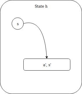
Look at this fucking diagram. It is actually the visualization of the
Static hin the definition above. The directed graph in the box is the stateful computation function which is wrapped. What it does in the definition is that thehis extrated using pattern matching and applied to the input statesto get a new state, which iss'in the graph above. Then thefafter>>=is applied to the value get from the output ofhand end up with another stateful computationg, which is them applied to new state. Just like following diagram.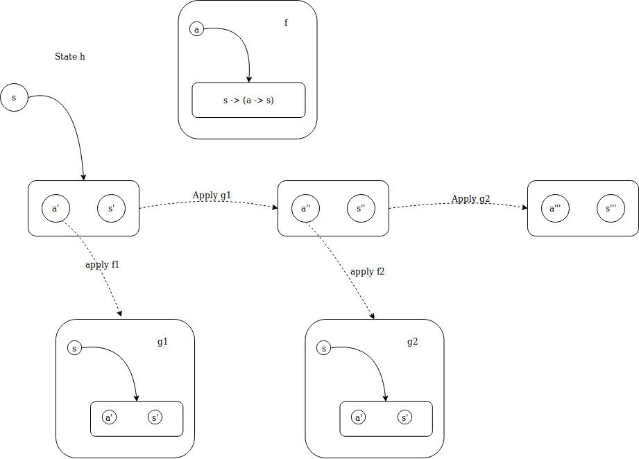
This diagram shows 2 sequential applications of
>>=for a state monad, which is like:State h >>= f1 >>= f2It can be seen that no matter how many functions are applied to it, it’s always in the form of taking a state and return a new state along with a value.
The Control.Monad.State module also provides a type class called MonadState with two useful functions, which are get and put. The get is defined as
get = State $ \s -> (s, s)
which returns the State with current state as its value. The put is defined as
put newState = State $ \s -> ((), newState)
But how does these shits work in an imperative looking do block with State Monad? If we look at the definition of >>= for State Monad, the chained function actually apply to the value of previous result and return a stateful computation that is applied to previous state. This means that things chained after get function are going to use the value returned by the function wrapped by get, in this case, the value is current state. The put is pretty much similar. Functions chained after put will see the new state set by the put function.